Global Wheat Detection | YOLOv8 Object Detection

Training Images

Bounding Boxes

Avg. Boxes per Image

Best Validation mAP

Best mAP @ IoU 50

Kaggle Score

Training Blueprint

Project Overview

The training notebook turns raw Kaggle annotations into a full KerasCV YOLOv8-M detector for dense wheat-head localization.

This project is a dense object-detection case study. Unlike simple classification, the model must find many small wheat heads inside each 1024×1024 image, often under background clutter, occlusion, different lighting, and field-source variation. The workflow uses YOLOv8-M with COCO pretraining, full-resolution image processing, ragged bounding-box tensors, KerasCV augmentation layers, a custom COCO metrics callback, and a three-stage optimization strategy.

Problem typeSingle-class object detection: every object is a wheat head, but the detector must predict many coordinates and confidence scores per image.

Dense scene challengeThe average annotated image contains 43.82 boxes, and the maximum reaches 116 boxes, creating heavy overlap and small-object pressure.

Two-notebook designTraining is isolated from inference. The best .keras artifact is uploaded to Kaggle Models, then reused by the submission notebook.

Infrastructure

Training Environment & Dependencies

Main libraries, accelerator setup, and reproducibility controls used by the YOLOv8 training notebook.

TensorFlow / KerasDistributed training, model compilation, callbacks, checkpointing, optimizer schedules, and the final .keras detector artifact.

KerasCVYOLOv8-M backbone and detector head, bounding-box aware augmentation, ragged box utilities, Focal Loss, CIoU box loss, and COCO-style metrics.

TPUStrategy / Accelerator RuntimeDetected TPU execution, global batch-size scaling, and steps_per_execution optimization for high-throughput 1024×1024 training.

Pandas, NumPy & JSONCSV parsing, annotation grouping, [x, y, w, h] to xyxy conversion, metadata handling, class mapping, and reproducible split preparation.

OpenCV, Matplotlib & SeabornImage inspection, bounding-box visualization, empty-image review, box-density plots, mosaic checks, and training diagnostics.

Scikit-learn UtilitiesTrain/validation splitting and controlled random-state handling, including the positive/negative sample separation used before dataset construction.

Data Intelligence

Dataset Structure & Detection Difficulty

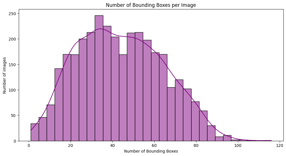
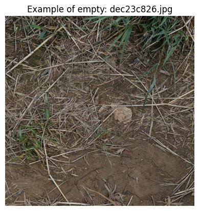
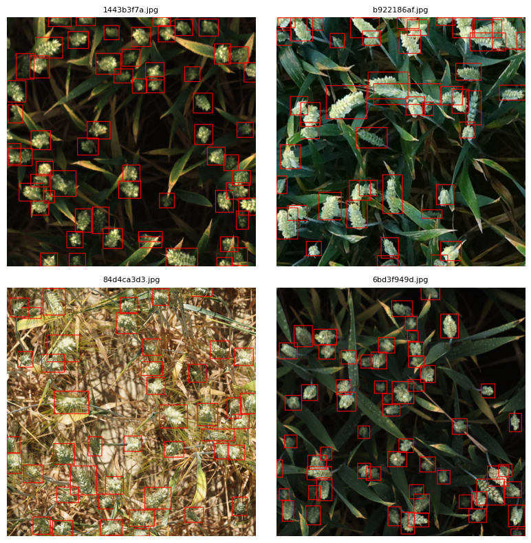
EDA revealed dense boxes, rare empty images, and small target objects in full-resolution field photographs.

Train / Test Images3422 / 10

Annotated Images3373

Empty Images49

Empty Fraction1.43%

EDA Component	Measured Value	Design Impact
`image_shape`	1024×1024×3	High resolution is preserved because wheat heads are small and spatial details matter.
`bbox_count`	147,793 annotations	The detector sees many positive boxes and needs efficient dense prediction.
`boxes_per_image`	mean 43.82 · std 20.37 · max 116	WBF/TTA is useful because crowded scenes produce duplicate and overlapping predictions.
`bbox_width`	mean 84.44 · median 78 px	Small-object sensitivity is essential; FPN-style multi-scale features help.
`bbox_height`	mean 76.93 · median 71 px	Boxes are compact relative to the full image, so aggressive downscaling would lose signal.
`negative_samples`	49 images without annotations	Empty images are added only to training to teach background rejection.

Bounding box density distribution — many images contain 30–60 objects, with a long dense tail

Negative sample — no visible wheat head annotation

Training samples with ground-truth boxes — confirms annotation conversion and box alignment

Model Mechanics

YOLOv8-M Architecture, Losses & Detection Logic

A COCO-pretrained one-stage detector is adapted to the single wheat-head class using KerasCV.

One-Stage YOLO Detection

YOLOv8

YOLO predicts object coordinates and confidence in one forward pass, making it suitable for dense scenes where many boxes must be produced quickly. In this notebook, the KerasCV detector uses YOLOV8Backbone.from_preset('yolo_v8_m_backbone_coco') and a YOLOV8Detector head.

Feature Pyramid Depth

FPN 3

The detector uses fpn_depth=3, allowing high-level semantics and lower-level spatial detail to interact. This matters because wheat heads can be small, partially hidden, and densely packed.

Focal Loss

Classification

$$FL(p_t)=-\alpha_t(1-p_t)^\gamma\log(p_t)$$

Focal loss reduces the dominance of easy background predictions and gives more weight to hard wheat-head examples in cluttered scenes.

CIoU Box Loss

Localization

$$\mathcal{L}_{CIoU}=1-IoU+\frac{\rho^2(b,b^{gt})}{c^2}+\alpha v$$

Complete IoU considers overlap, center distance, and aspect-ratio consistency, helping the model learn tighter bounding boxes.

Model Configuration

Core model parameters

Input size: 1024×1024
Classes: 1 wheat-head class
Bounding box format: xyxy
Backbone: yolo_v8_m_backbone_coco
Visible backbone parameter count in summary: 11,872,464

Training Stability

Optimization controls

Optimizer: AdamW
Weight decay: 1e-3
Gradient clipping: global_clipnorm=10.0
BatchNorm layers frozen to avoid unstable running statistics with small batches

Input Pipeline

Ragged Tensors, Splits & Augmentation Strategy

The notebook prepares variable-length boxes with tf.data and uses phase-specific augmentation strength.

Parse raw annotationsKaggle boxes are converted from [x, y, w, h] to [x_min, y_min, x_max, y_max].

Group boxes by imageEach image becomes one dictionary with an image path and a variable number of boxes.

Train/validation splitPositive samples are split 80/20 with seed 28; empty images are inserted into the training set only.

Ragged batchingBoxes and classes are stored as ragged tensors because every image has a different number of objects.

Prefetch pipelinetf.data.AUTOTUNE and prefetching overlap CPU loading/augmentation with GPU training.

Strong Augmentation

Warmup / early robustness

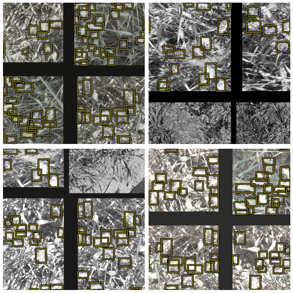
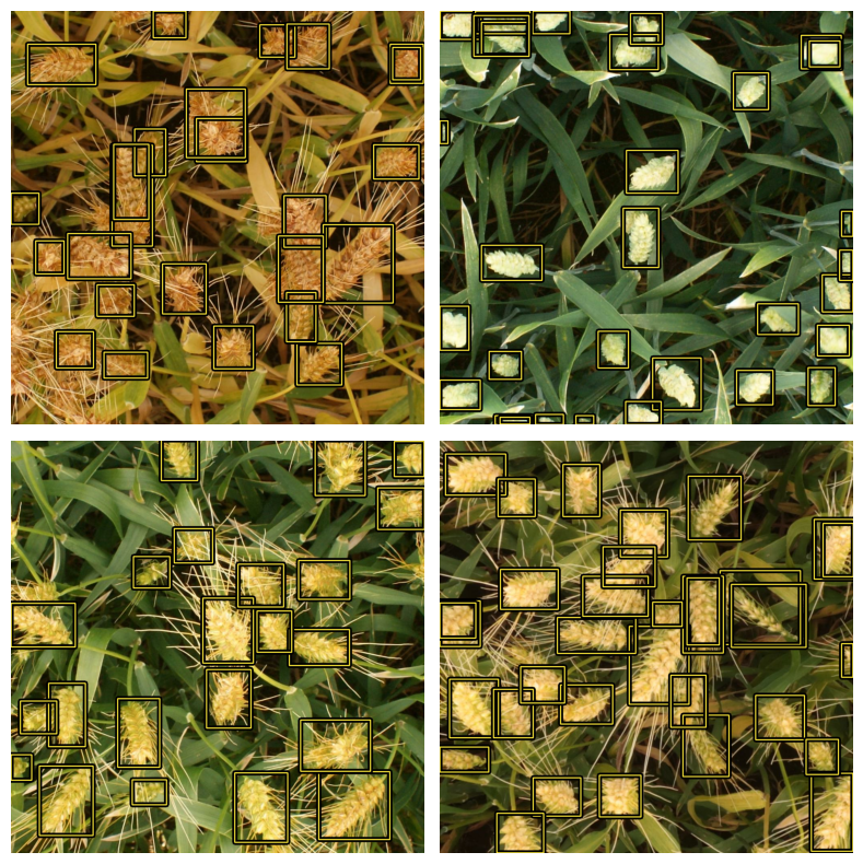
Uses JitteredResize(0.9–1.1), Mosaic, horizontal flip, strong color jitter, and color degeneration. Mosaic is especially useful because it exposes the model to more object arrangements and denser context per batch.

Light Augmentation

Mid/Fine-tune stability

Uses reduced scale jitter 0.95–1.05, horizontal flip, milder color jitter, and lower color degeneration. This keeps the training distribution closer to validation while still preventing overfitting.

strong_augmentation.py

# Warmup / early training: maximize variation
augmenter_strong = tf.keras.Sequential([
    keras_cv.layers.JitteredResize(
        target_size=IMG_SIZE,
        scale_factor=(0.9, 1.1),
        bounding_box_format="xyxy"
    ),
    keras_cv.layers.Mosaic(
        bounding_box_format="xyxy", name="mosaic"
    ),
    keras_cv.layers.RandomFlip(
        mode="horizontal", bounding_box_format="xyxy"
    ),
    keras_cv.layers.RandomColorJitter(
        value_range=(0, 255),
        brightness_factor=0.2,
        contrast_factor=0.2,
        saturation_factor=0.2,
        hue_factor=0.1,
    ),
    keras_cv.layers.RandomColorDegeneration(
        factor=(0.2, 0.7), seed=SEED
    ),
])

dataset_factory.py

# KerasCV needs ragged boxes: each image has a different object count
def create_strong_dataset(records, batch_size=BATCH_SIZE):
    paths, classes, boxes = prepare_inputs(records)
    ds = tf.data.Dataset.from_tensor_slices((paths, classes, boxes))
    ds = ds.shuffle(BUFFER_SHUFFLE_SIZE)
    ds = ds.map(load_dataset, num_parallel_calls=AUTO)
    ds = ds.ragged_batch(batch_size, drop_remainder=True)
    ds = ds.map(augmenter_strong, num_parallel_calls=AUTO)
    ds = ds.map(dict_to_tuple, num_parallel_calls=AUTO)
    return ds.prefetch(AUTO)

# Mid/fine-tune swaps to lighter augmentation
def create_light_dataset(records, is_training=False):
    augmenter = augmenter_light if is_training else augmenter_val
    # same load → ragged_batch → augment → tuple → prefetch path
    return build_dataset(records, augmenter, is_training)

Mosaic augmentation output — multiple scenes merged with transformed wheat-head boxes

Ground-truth box samples — confirms ragged tensors and box transforms stay aligned

Optimization Strategy

Three-Phase Training Diagnostics

Warmup stabilizes the head, mid-tune specializes deeper features, and fine-tune reaches the final mAP ceiling.

Phase 1

Warmup Head TrainingEpochs 1–10. Backbone frozen, BatchNorm frozen, warmup LR 1e-3. The head learns wheat localization without disturbing pretrained COCO features.

mAP Start0.2530

Best mAP0.4617

Box Loss Δ-0.7475

Phase 2

Mid-Tune Partial SpecializationEpochs 11–30. Deeper tuning with cosine decay improves stricter localization and pushes validation mAP above 0.50.

Start mAP0.4816

Peak mAP0.5063

mAP@750.5262

Phase 3

Full Fine-Tune RefinementEpochs 31–51 logged. Full backbone refinement with low LR 1e-5 gives smaller but valuable improvements, especially for tiny/distant wheat heads.

Best Epoch43

Best mAP0.5127

Best mAP@500.8704

Metric	Warmup Best	Mid-Tune Peak	Fine-Tune Peak	Meaning
`Validation mAP`	0.4617	0.5063	0.5127	Main COCO-style detection quality metric.
`mAP@50`	0.8272	0.8686	0.8704	Loose IoU localization; strong indication the detector finds wheat heads.
`mAP@75`	0.4617	0.5262	0.5331	Stricter localization; improved during deeper tuning.
`Training box loss`	1.2328	1.0480	0.9734	Regression loss continued declining through fine-tuning.

Diagnostic Breakdown: The biggest improvement happened during warmup (+0.2087 mAP), confirming the pretrained detector adapted quickly. Mid-tune crossed the 0.50 mAP threshold and improved stricter box alignment. Fine-tune added a smaller but important final gain to 0.5127, which is expected for a dense small-object competition where overlap and occlusion create a practical ceiling.

Configuration Layer

Model Parameters & Training Controls

The notebook keeps the detector close to the competition setup: full 1024×1024 images, one wheat-head class, AdamW regularization, and staged learning rates.

Parameter Group	Notebook Value	Implementation Role
`IMG_SIZE`	`(1024, 1024)`	Full-resolution training keeps wheat heads large enough for reliable box regression.
`NUM_CLASSES`	`1`	Single detector class: wheat head. The challenge is localization density, not class variety.
`bounding_box_format`	`xyxy`	All training, augmentation, metrics, TTA reversal, and WBF logic use xmin/ymin/xmax/ymax.
`backbone preset`	`yolo_v8_m_backbone_coco`	COCO-pretrained YOLOv8-M backbone provides general object features before agricultural fine-tuning.
`backbone params`	`11,872,464`	The visible backbone summary confirms the medium preset size used for this portfolio detector.
`fpn_depth`	`3`	Feature Pyramid depth controls multi-scale detection refinement for small, medium, and larger wheat heads.
`BATCH_SIZE_PER_REPLICA`	`4`	Chosen because 1024×1024 object-detection tensors are memory heavy.
`BUFFER_SHUFFLE_SIZE`	`512`	Randomizes training order without huge memory overhead.
`GLOBAL_CLIPNORM`	`10.0`	Clips gradient norm to reduce exploding updates during dense box optimization.
`optimizer`	`AdamW`	Combines Adam-style adaptive learning with decoupled weight decay for regularized fine-tuning.
`classification_loss`	`FocalLoss()`	Down-weights easy background/low-value examples and emphasizes hard wheat-head detections.
`box_loss`	`ciou`	Optimizes overlap, center distance, and aspect-ratio consistency for tighter boxes.
`steps_per_execution`	`32 on TPU else 1`	Improves TPU execution efficiency while keeping GPU/CPU behavior simple.
`WARMUP_LR`	`1e-3`	Fast detector-head adaptation while the backbone is frozen.
`FINE_TUNE_BB_LR`	`1e-4`	Partial backbone tuning from `stack4_downsample_conv` with cosine decay.
`FINE_TUNE_MODEL_LR`	`1e-5`	Full fine-tuning with tiny updates for final localization refinement.
`epochs`	`10 → 30 → 80`	Warmup, mid-tune, and fine-tune use increasing patience and decreasing update size.

Detector Setup

YOLOv8-M in KerasCV

The implementation builds a YOLOV8Detector around a COCO-pretrained medium backbone, sets num_classes=1, keeps the box format consistent as xyxy, and uses fpn_depth=3 for multi-scale feature aggregation.

Training Control

Why staged learning rates?

The notebook does not unfreeze everything at once. It first trains the detector head, then unfreezes deeper backbone layers, then performs full low-LR refinement while keeping BatchNorm frozen for stability.

Implementation

Core Training Code

A compact view of the central setup: YOLOv8-M, COCO weights, AdamW, focal classification loss, CIoU box loss, and staged optimization.

01_build_detector.py

# COCO-pretrained YOLOv8-M detector for one wheat-head class
def create_detector():
    backbone = keras_cv.models.YOLOV8Backbone.from_preset(
        "yolo_v8_m_backbone_coco"
    )
    return keras_cv.models.YOLOV8Detector(
        backbone=backbone,
        num_classes=1,
        bounding_box_format="xyxy",
        fpn_depth=3,
    )

with strategy.scope():
    model = create_detector()
    model.backbone.trainable = False

    # Keep BatchNorm stable with small high-res batches
    for layer in model.backbone.layers:
        if isinstance(layer, tf.keras.layers.BatchNormalization):
            layer.trainable = False

02_compile_warmup.py

# Phase 1: train detection head/neck while backbone is frozen
optimizer = tf.keras.optimizers.AdamW(
    learning_rate=WARMUP_LR,     # 1e-3
    weight_decay=1e-3,
    beta_1=0.9,
    beta_2=0.999,
    global_clipnorm=GLOBAL_CLIPNORM,
)

model.compile(
    optimizer=optimizer,
    classification_loss=keras_cv.losses.FocalLoss(),
    box_loss="ciou",
    steps_per_execution=32 if is_tpu else 1,
)

history = model.fit(
    train_strong_dataset.repeat(),
    validation_data=val_dataset.repeat(),
    epochs=WARMUP_EPOCH,
    callbacks=[coco_cb, early_stopping_cb, reduce_lr_cb],
    steps_per_epoch=steps_per_epoch,
    validation_steps=validation_steps,
)

03_partial_unfreeze.py

# Phase 2: reload warmup checkpoint and unfreeze only deep backbone layers
START_UNFREEZE_LAYER_NAME = "stack4_downsample_conv"
model = tf.keras.models.load_model(
    "/kaggle/input/wheat-detection/keras/warmup/1/warmup_best_model.keras",
    custom_objects={
        "YOLOV8Detector": keras_cv.models.YOLOV8Detector,
        "YOLOV8Backbone": keras_cv.models.YOLOV8Backbone,
    },
)

model.backbone.trainable = True
unfreeze = False
for layer in model.backbone.layers:
    if layer.name == START_UNFREEZE_LAYER_NAME:
        unfreeze = True
    layer.trainable = unfreeze
    if isinstance(layer, tf.keras.layers.BatchNormalization):
        layer.trainable = False

lr = tf.keras.optimizers.schedules.CosineDecay(
    initial_learning_rate=FINE_TUNE_BB_LR,  # 1e-4
    decay_steps=steps_per_epoch * (INTERMEDIATE_EPOCH - WARMUP_EPOCH),
    alpha=0.1,
)

04_full_finetune_phase3.py

# Phase 3: full unfreezing + very low LR refinement
model = tf.keras.models.load_model(
    "/kaggle/input/wheat-detection/keras/warmup/2/midtune_best_model.keras",
    custom_objects={
        "YOLOV8Detector": keras_cv.models.YOLOV8Detector,
        "YOLOV8Backbone": keras_cv.models.YOLOV8Backbone,
    },
)

model.backbone.trainable = True
for layer in model.backbone.layers:
    layer.trainable = True
    if isinstance(layer, tf.keras.layers.BatchNormalization):
        layer.trainable = False

for layer in model.layers:
    if isinstance(layer, tf.keras.layers.BatchNormalization):
        layer.trainable = False

lr = tf.keras.optimizers.schedules.CosineDecay(
    initial_learning_rate=FINE_TUNE_MODEL_LR,  # 1e-5
    decay_steps=steps_per_epoch * (FINAL_EPOCH - INTERMEDIATE_EPOCH),
    alpha=0.1,
)

model.compile(
    optimizer=tf.keras.optimizers.AdamW(
        learning_rate=lr, weight_decay=1e-4,
        beta_1=0.9, beta_2=0.999,
        global_clipnorm=GLOBAL_CLIPNORM,
    ),
    classification_loss=keras_cv.losses.FocalLoss(),
    box_loss="ciou",
    steps_per_execution=32 if is_tpu else 1,
)

Implementation takeaway: the notebook treats training as a controlled optimization path, not one giant fit() call. Phase 1 protects COCO features, Phase 2 adapts high-level backbone layers, and Phase 3 fully unfreezes the detector with tiny cosine-decayed updates while BatchNorm remains frozen.

Inference Blueprint

Saved Model Loading & Submission Pipeline

The inference notebook stays separate from training: it loads the Kaggle Model artifact, verifies predictions, applies TTA, fuses boxes with WBF, and writes the competition submission.

The final detector is loaded from /kaggle/input/wheat-detection/keras/warmup/3/finetune_best_model.keras using KerasCV custom objects. The notebook uses 1024×1024 inference resolution, CONF_THRESHOLD = 0.40, IOU_THRESHOLD = 0.50, and Test-Time Augmentation before Weighted Boxes Fusion. The resulting submission.csv follows the Kaggle format: confidence xmin ymin width height.

Model sourceKaggle Model artifact loaded without retraining, keeping inference lightweight and reproducible.

TTA viewsIdentity, horizontal flip, vertical flip, and multiple photometric jitter variants are combined.

Final scoreThe submission workflow reached a Kaggle score of 0.6055.

Inference Infrastructure

Inference Libraries & Dependencies

Runtime tools used to load the saved detector, run TTA, fuse duplicate boxes, and export the Kaggle submission file.

TensorFlow / KerasLoads the saved finetune_best_model.keras artifact with KerasCV custom objects and performs batched prediction on test images.

KerasCVRestores YOLOV8Detector and YOLOV8Backbone, preserves the xyxy bounding-box convention, and supports inference visualization.

Weighted Boxes FusionThe ensemble_boxes WBF utility merges duplicate detections from identity, flip, and color-jitter TTA views into cleaner final boxes.

TensorFlow Image OpsHorizontal flip, vertical flip, color jitter, and coordinate-reversal helpers create the multi-view TTA prediction set.

Pandas & NumPyPrediction arrays, confidence filtering, WBF normalization/denormalization, and final submission.csv formatting.

Matplotlib / OpenCVDebug prediction plots, initial inference checks, and final TTA + WBF visual verification before submission.

Baseline Prediction

Initial Inference & Confidence Filtering

Before TTA/WBF, the notebook validates model loading and raw prediction behavior on test images.

Prediction Utility

Single-image detection

The helper function expands a single image to batch shape, calls model.predict(), and keeps only detections above the confidence threshold. The output remains in KerasCV dictionary format with boxes, classes, and confidence.

Visual Check

Why this step matters

Initial prediction visualization confirms that the saved model artifact loads correctly, bounding boxes are in the expected xyxy coordinate space, and the threshold is reasonable before adding TTA complexity.

Initial inference example — raw YOLOv8 detections before final TTA/WBF fusion

Robust Prediction

Test-Time Augmentation Strategy

TTA increases viewpoint and lighting coverage while preserving final coordinates through reversal functions.

Horizontal Flip Reversal

Geometry

$$x_{min}^\prime = W-x_{max},\quad x_{max}^\prime = W-x_{min}$$

Horizontal-flip predictions are mapped back by reversing x-coordinates around the image width. Y-coordinates remain unchanged.

Vertical Flip Reversal

Geometry

$$y_{min}^\prime = H-y_{max},\quad y_{max}^\prime = H-y_{min}$$

Vertical-flip predictions are restored by reversing y-coordinates around the image height. X-coordinates remain unchanged.

Photometric Variants

Lighting

Four random color-jitter views adjust hue, contrast, saturation, and brightness. Because these are non-geometric transforms, boxes do not need coordinate reversal.

Aggregation Before Fusion

TTA

The notebook logs every TTA sequence and concatenates all boxes, scores, and classes. One debug image produced 295 candidate boxes before WBF, demonstrating why fusion is required.

tta_sequences.py

# 7 executed views: identity, flips, and color perturbations
TTA_SEQUENCES = [
    (lambda img: img, lambda boxes: boxes),
    (tf.image.flip_left_right, reverse_h_flip),
    (tf.image.flip_up_down, reverse_v_flip),
    (lambda img: random_color_jitter(img), lambda boxes: boxes),
    (lambda img: random_color_jitter(img), lambda boxes: boxes),
    (lambda img: random_color_jitter(img), lambda boxes: boxes),
    (lambda img: random_color_jitter(img), lambda boxes: boxes),
]

# Geometric TTA must reverse coordinates back to original space
def reverse_h_flip(boxes, image_width=IMG_SIZE[1]):
    xmin, ymin, xmax, ymax = tf.split(boxes, 4, axis=-1)
    return tf.concat([image_width - xmax, ymin, image_width - xmin, ymax], axis=-1)

tta_aggregation.py

def run_tta(model, image_tensor, conf_threshold=0.40):
    collected = []
    for augment_fn, reverse_fn in TTA_SEQUENCES:
        aug_img = augment_fn(image_tensor)
        pred = model.predict(tf.expand_dims(aug_img, 0), verbose=0)
        keep = pred["confidence"] > conf_threshold

        boxes = tf.ragged.boolean_mask(pred["boxes"], keep)[0]
        scores = tf.ragged.boolean_mask(pred["confidence"], keep)[0]
        classes = tf.ragged.boolean_mask(pred["classes"], keep)[0]

        if tf.shape(boxes)[0] > 0:
            boxes = reverse_fn(boxes)
            collected.append((boxes.numpy(), scores.numpy(), classes.numpy()))

    return concatenate_tta_predictions(collected)

Post-Processing

Weighted Boxes Fusion & Submission Formatting

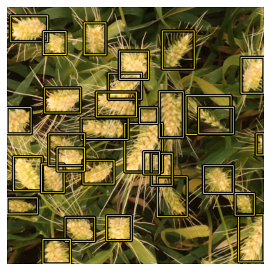
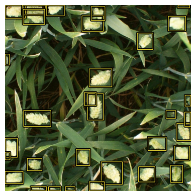
WBF merges duplicate TTA predictions instead of simply discarding them like standard NMS.

Weighted Box Coordinates

WBF

$$x_{fused}=\frac{\sum_i s_i x_i}{\sum_i s_i}$$

WBF uses prediction confidence as weights, so repeated detections from multiple TTA views pull the final coordinate toward the strongest consensus.

Why WBF Over NMS?

Dense Scenes

NMS removes boxes. WBF combines them. In wheat images, several TTA views may detect the same head with slightly shifted boxes, so fusion can produce cleaner localization.

Image	TTA Candidate Boxes	After WBF	After Final Filter
`debug_image`	295	32	32
`796707dd7`	229	31	31
`2fd875eaa`	335	32	32
`cc3532ff6`	255	30	30
`53f253011`	297	32	32
`51f1be19e`	466	51	51

weighted_boxes_fusion.py

def fuse_boxes(boxes, scores, classes, img_size=IMG_SIZE):
    # WBF expects normalized coordinates in [0, 1]
    boxes_norm = boxes / img_size[0]
    fused_boxes, fused_scores, fused_labels = weighted_boxes_fusion(
        [boxes_norm.tolist()],
        [scores.tolist()],
        [classes.astype(float).tolist()],
        weights=None,
        iou_thr=0.50,
        conf_type="max",
        skip_box_thr=0.0001,
    )
    return np.array(fused_boxes) * img_size[0], np.array(fused_scores)

submission_string.py

def to_kaggle_prediction_string(fused_boxes, fused_scores):
    keep = fused_scores >= 0.40
    parts = []
    for box, score in zip(fused_boxes[keep], fused_scores[keep]):
        xmin, ymin, xmax, ymax = box
        width = xmax - xmin
        height = ymax - ymin
        parts.extend([
            f"{score:.4f}",
            str(int(xmin)), str(int(ymin)),
            str(int(width)), str(int(height)),
        ])
    return " ".join(parts)

Inference Visuals

Final TTA + WBF Output Examples

Final predictions are cleaner after coordinate reversal, confidence filtering, and box fusion.

Final TTA + WBF example 1 — fused wheat-head predictions

Final TTA + WBF example 2 — dense field localization after fusion

Conclusion

Project Synthesis & Roadmap

The final workflow separates heavy training from robust inference and is ready for future detector experiments.

Training result: The staged YOLOv8-M workflow achieved a best recorded validation mAP of 0.5127 at epoch 43, with 0.8704 mAP@50. The strongest gains came from warmup and mid-tune; fine-tuning gave smaller but meaningful small-object improvements.

Inference result: The final notebook applies seven executed TTA views per test image, reverses geometric transforms, uses WBF with IoU threshold 0.50, and exports a Kaggle-ready submission.csv, with the final Kaggle score recorded as 0.6055.

Future directions:

Try larger YOLO presets or ensemble multiple checkpoints.
Experiment with CutMix, MixUp, Random Erasing, and tuned Mosaic probability.
Run threshold sweeps for confidence and WBF IoU to optimize public/private leaderboard behavior.
Compare WBF with Soft-NMS and class-aware NMS for dense wheat clusters.

Global Wheat Detection: YOLOv8 Dense Field Localization